Technical validation

This notebook will perform a theoretical analysis of measured curvatures on an ideal ellipsoid. In the second part, it compares the outputs of measurements done with napari-stress to those of the legacy-version STRESS as well as .

import numpy as np
import matplotlib.pyplot as plt
import matplotlib as mpl
import os
import napari
import pandas as pd
import vedo
import seaborn as sns
from napari_stress import sample_data, reconstruction, measurements

Benchmarking

In this section, we benchmark the performance of napari-stress. This is done by performing two tests on synthetic image data of a blurry ellipsoid:

• We reconstruct the pointcloud with napari-stress. We then measure the deviation of the recovered point cloud from the original pointcloud.

• We measure the mean curvatures of the ellipsoid with napari-stress. We then compare the measured mean curvatures to the theoretical mean curvatures of the same ellipsoid.

Relative deviation of pointcloud

In the next cell, we create a list of major axis lengths for which we want to calculate the theoretical mean curvatures. The different set of major axis lengths is used to test the robustness of the mean curvature calculation and corresponds to ellipsoids of different aspect ratios.

The relative deviation of the pointcloud is calculated as the average deviation of every traced point from its corresponding correct location in x,y and z divided by the respective point’s true location in x,y and z. In order to calculate the corresponding location of a point on the surface of a given ellipsoid, we transform both te query point and the ellipsoid into a coordinate system where the ellipsoid is centered at the origin and has major axes lengths of 1. In this coordinate system, the location of a point on the surface of the ellipsoid can be found by calculating its coordinates in polar coordinates; its elevation and azimuth can be kept and the radius is replaced by the major axis length of the ellipsoid. The point is then transformed back into the original coordinate system.

In formulas:

Query point: \(\vec{p}\), Ellipsoid major axes: \(a, b, c\), Ellipsoid center: \(\vec{c}\)

\begin {align} \vec{p}’ &= \underbrace{\begin{bmatrix} \frac{1}{a} & 0 & 0\ 0 & \frac{1}{b} & 0\ 0 & 0 & \frac{1}{c} \end{bmatrix}}{T} \cdot(\vec{p} - \vec{c}) = \begin {bmatrix} x’ \ y’ \ z’ \end{bmatrix} = \begin {bmatrix} r’\ \theta’ \ \phi’ \end{bmatrix} \ \vec{p{sphere}}’ &= \begin{bmatrix} 1\ \theta’ \ \phi’ \end{bmatrix}\ \vec{p_{ellipsoid}} &= T^{-1} \cdot \vec{p_{sphere}}’ + \vec{c} \end{align}

def project_point_on_ellipse_surface(query_point: np.ndarray,
                                     a: float,
                                     b: float,
                                     c: float,
                                     center: np.ndarray) -> np.ndarray:
    """Project a point on the surface of an ellipsoid.

    Parameters
    ----------
    query_point : np.ndarray
        Point to project on the surface of the ellipsoid.
    a : float
        Length of the first axis of the ellipsoid.
    b : float
        Length of the second axis of the ellipsoid.
    c : float
        Length of the third axis of the ellipsoid.
    center : np.ndarray
        Center of the ellipsoid.

    Returns
    -------
    np.ndarray
        Point on the surface of the ellipsoid.
    """
    # transformation matrix to turn ellipsoid into a sphere
    T = np.array([[1/a, 0, 0],
                  [0, 1/b, 0],
                  [0, 0, 1/c]])
    
    # transform query point to coordinate system in which ellipsoid is a sphere
    transformed_query_point = np.dot(query_point - center, T)

    # transform query point into spherical coordinates
    transformed_query_point_spherical = vedo.transformations.cart2spher(transformed_query_point[2],
                                                              transformed_query_point[1],
                                                              transformed_query_point[0])
    
    # replace radius of query point with radius of sphere, which in this coordinate 
    # system is always 0.5
    point_on_transformed_ellipse_surface = np.array([0.5, 
                                                     transformed_query_point_spherical[1],
                                                     transformed_query_point_spherical[2]])
    
    # transform point on sphere back to cartesian coordinates
    point_on_transformed_ellipse_surface = vedo.transformations.spher2cart(*point_on_transformed_ellipse_surface)[::-1]
    point_on_ellipse_surface = np.dot(point_on_transformed_ellipse_surface, np.linalg.inv(T)) + center

    return point_on_ellipse_surface

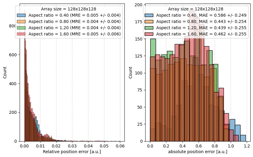
We now calculate the relative deviation of the pointcloud for several aspect ratios. The results are shown in the following plot; We find that the relative deviation is below 1% for all aspect ratios and the absolute deviation is consistenly below 1 pixel. The legend shows the aspect ratio of the ellipsoid as well as mean relative errors (MRE) and mean absolute errors (MAE) in pixels.

import matplotlib as mpl
mpl.style.use('default')

size = 128
b, c = 0.5, 0.5
number_of_ellipsoids = 4

fig, axes = plt.subplots(ncols = 2, figsize=(10,6))

for a in np.linspace(0.2, 0.8, number_of_ellipsoids):
    
    ellipsoid = sample_data.make_blurry_ellipsoid(a, b, c, size, definition_width=10)[0]
    results_reconstruction = reconstruction.reconstruct_droplet(ellipsoid, voxelsize=np.array([1,1,1]), use_dask=False,
                                                            resampling_length=3, interpolation_method='linear', trace_length=10, sampling_distance=1)

    # calculate each point's distance to the surface of the ellipsoid
    distances = []
    ellipse_points = []
    for pt in results_reconstruction[3][0]:
        ellipse_points.append(project_point_on_ellipse_surface(pt, a*size, b*size, c*size, np.array([size/2, size/2, size/2])))
        distances.append(np.linalg.norm(pt - ellipse_points[-1]))
    distances = np.array(distances).flatten()

    # relative position error in x, y and z direction
    relative_position_error = np.abs(results_reconstruction[3][0] - ellipse_points) / ellipse_points
    relative_position_error = relative_position_error.flatten()

    # plot distance distribution
    sns.histplot(data=relative_position_error, ax=axes[0],
                label='Aspect ratio = {:.2f} (MRE = {:.3f} +/- {:.3f})'.format(a/b, np.mean(relative_position_error), np.std(relative_position_error)),
                alpha=0.5)
    sns.histplot(data=distances, ax=axes[1], label='Aspect ratio = {:.2f}, MAE = {:.3f} +/- {:.3f}'.format(a/b, np.mean(distances), np.std(distances)), alpha=0.5)

axes[0].set_xlabel('Relative position error [a.u.]')
axes[0].grid(which='major', axis='x', linestyle='--', alpha=0.5)
axes[0].legend(title='Array size = {size}x{size}x{size}'.format(a*size/2, b*size/2, c*size/2, size=size))
axes[1].set_xlabel('absolute position error [a.u.]')
axes[1].grid(which='major', axis='x', linestyle='--', alpha=0.5)
axes[1].legend(title='Array size = {size}x{size}x{size}'.format(a*size/2, b*size/2, c*size/2, size=size))

<matplotlib.legend.Legend at 0x165530f0dc0>

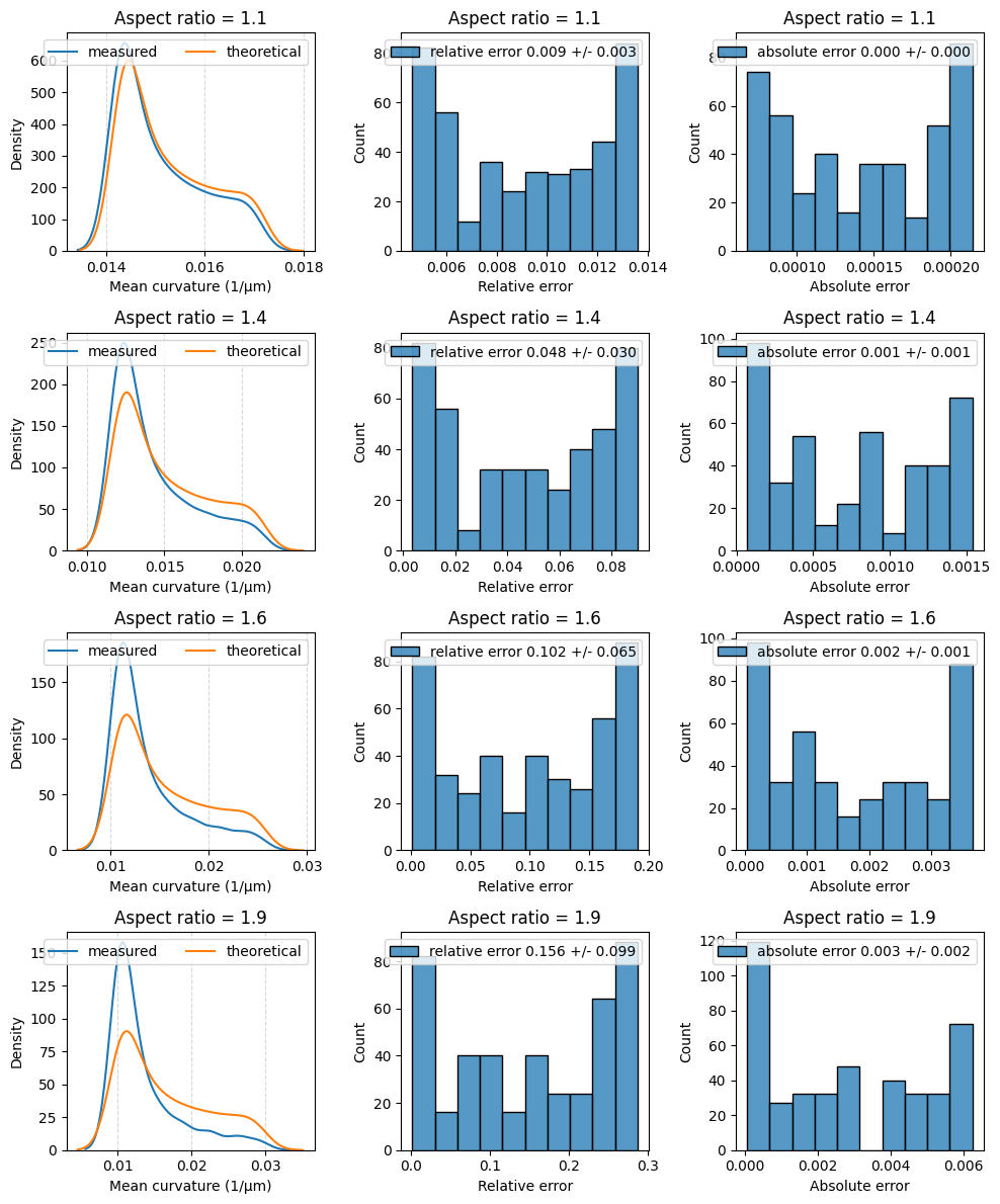
Relative and absolute mean curvature deviation

Mean curvature \(H\) on an ellipse is given by the following formula:

\(H = \frac{a b c [3(a^2+b^2) + 2c^2 + (a^2 + b^2 -2c^2)cos(2\phi) - 2(a^2 - b^2)cos(2\theta)sin^2(\phi)]}{8[a^2b^2cos^2(\phi) + c^2(b^2 cos^2(\theta) + a^2 sin^2 (\theta)) sin^2\phi]^{3/2}}\)

where a, b and c are the major axis length of the ellipsoid. The angles \(\theta\) and \(\phi\) denote the location on the surface of the ellipsoid in polar coordinates (azimuth \(\theta \in [0, 2\pi]\), elevation \(\phi \in [0, \pi]\)). We can thus compare all measurements of mean curvature on an ellipsoid to the “true” mean curvature.

def theoretical_mean_curvature_on_pointcloud(a, b, c, pointcloud) -> float:
    """Theoretical mean curvature of an ellipsoid.

    Parameters
    ----------
    a : float
        Length of the first semi-axis.
    b : float
        Length of the second semi-axis.
    c : float
        Length of the third semi-axis.
    elevation : float
        Angular position of sample on ellipsoid surface
    azimuth : float
        Equatorial position of sample on ellipsoid surface
    """

    pointcloud = pointcloud - pointcloud.mean(axis=0)[None, :]
    
    pointcloud_spherical = vedo.transformations.cart2spher(pointcloud[:, 2], pointcloud[:, 1], pointcloud[:, 0])
    elevation = pointcloud_spherical[1]
    azimuth = pointcloud_spherical[2]
    
    above = a * b * c * (3 * (a**2 + b**2) + 2*c**2 + (a**2 + b**2 - 2*c**2)*np.cos(2*elevation) - 2*(a**2 - b**2)*np.cos(2*azimuth) * np.sin(elevation)**2)
    below = 8 * (a**2 * b**2 *np.cos(elevation)**2 + c**2 * (b**2 * np.cos(azimuth)**2 + a**2 * np.sin(azimuth)**2) * np.sin(elevation)**2)**(3/2)
    return above/below

Again, we calculate the relative and absolute mean curvature deviation for several aspect ratios. We show the distribution of mean curvatures from the ideal ellipsoid and the measured mean curvatures as well as the distribution of the relative and absolute mean curvature deviation.

size = 256
b, c = 0.5, 0.5
number_of_ellipsoids = 4

fig, axes = plt.subplots(nrows=number_of_ellipsoids, ncols=3, figsize=(10,3 * number_of_ellipsoids))

for idx, a in enumerate(np.linspace(0.55, 0.95, number_of_ellipsoids)):
    
    ellipsoid = sample_data.make_blurry_ellipsoid(a, b, c, size, definition_width=10)[0]
    results_reconstruction = reconstruction.reconstruct_droplet(ellipsoid, voxelsize=np.array([1,1,1]), use_dask=False,
                                                            resampling_length=3, interpolation_method='linear', trace_length=10, sampling_distance=1)
    results_measurement = measurements.comprehensive_analysis(results_reconstruction[3][0], max_degree=20, n_quadrature_points=434, gamma=5)

    mean_curvature_measured = results_measurement[3][1]['features']['mean_curvature']
    mean_curvature_theoretical = theoretical_mean_curvature_on_pointcloud(c * size/2, b * size/2, a * size/2,
                                                                          results_measurement[4][0])
    relative_difference = np.abs(mean_curvature_measured - mean_curvature_theoretical) / mean_curvature_theoretical
    absolute_difference = np.abs(mean_curvature_measured - mean_curvature_theoretical)
    
    sns.kdeplot(data=mean_curvature_measured, ax=axes[idx, 0], label='measured')
    sns.kdeplot(data=mean_curvature_theoretical, ax=axes[idx, 0], label='theoretical')
    sns.histplot(data=relative_difference, ax=axes[idx, 1], label='relative error {:.3f} +/- {:.3f}'.format(np.mean(relative_difference), np.std(relative_difference)))
    sns.histplot(data=absolute_difference, ax=axes[idx, 2], label='absolute error {:.3f} +/- {:.3f}'.format(np.mean(absolute_difference), np.std(absolute_difference)))

    for ax in axes[idx, :]:
        axes[idx, 0].set_xlabel('Mean curvature (1/µm)')
        axes[idx, 1].set_xlabel('Relative error')
        axes[idx, 2].set_xlabel('Absolute error')
        axes[idx, 0].grid(which='major', axis='x', linestyle='--', alpha=0.5)
        ax.set_title('Aspect ratio = {:.1f}'.format(a/b))
        ax.legend(ncols=2)
    
fig.tight_layout()

Error in PyGeodesicAlgorithmExact.geodesicDistances: zero-size array to reduction operation minimum which has no identity
Error in PyGeodesicAlgorithmExact.geodesicDistances: zero-size array to reduction operation minimum which has no identity
Error in PyGeodesicAlgorithmExact.geodesicDistances: zero-size array to reduction operation minimum which has no identity
Error in PyGeodesicAlgorithmExact.geodesicDistances: zero-size array to reduction operation minimum which has no identity

Legacy validation

In this section, we compare the results of the legacy version of STRESS to the results of napari-stress using the same synthetic data.

We compare three analysis workflows:

• Using the reconstruction and the measurement from STRESS

• Using the STRESS reconstruction and the measurement from napari-stress

• using the napari-stress reconstruction and the measurement from napari-stress

We compare the reconstruction and measured quantities for the following synthetic data:

• Ideal sphere

• Ideal ellipsoid

Comparisons:

For all workflows, we compare the following quantities:

• The reconstructed pointcloud: Since the reconstructed object should be perfectly spherical, we can convert the reconstructed pointcloud coordinates to spherical coordinates and compare the distribution of radii of both reconstructions.

• Measured mean curvatures: Similar to the distribution of measured radii, the measured mean curvatures should follow a similar and ideally narrow distributioin

• Total stress anisotropies: For an ideal sphere, these should be as close to zero as possible.

viewer = napari.Viewer()

Sphere

We begin with comparing measurements for the ideal sphere. For this we load the data that was created with all listed measurement approaches:

dataset = os.path.join('.', 'results_sphere')

pointcloud_stress0 = pd.read_csv(os.path.join(dataset, 'stress_analysis_and_stress_pointcloud', 'pointcloud.csv'), sep=',', header=None).to_numpy()
pointcloud_napari_stress0 = pd.read_csv(os.path.join(dataset, 'napari_stress_analysis_and_napari_stress_pointcloud', 'pointcloud.csv'), sep=' ', header=None).to_numpy()

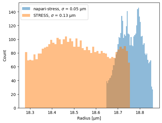
Radii

To better compare the two pointcouds visually, we can convert both to relative coordinates by subtracting the pointcloud’s center from every point:

pointcloud_stress0_centered = pointcloud_stress0 - pointcloud_stress0.mean(axis=0)[None, :]
pointcloud_napari_stress0_centered = pointcloud_napari_stress0 - pointcloud_napari_stress0.mean(axis=0)[None, :]

We can convert the points into spherical coordinates and measure the distribution of radii. For an ideal sphere, the standard deviation \(\sigma\) of the radii should be zero:

r_ns, phi_ns, theta_ns = vedo.transformations.cart2spher(pointcloud_napari_stress0_centered[:, 0], pointcloud_napari_stress0_centered[:, 1], pointcloud_napari_stress0_centered[:, 2])
r_s, phi_s, theta_s = vedo.transformations.cart2spher(pointcloud_stress0_centered[:, 0], pointcloud_stress0_centered[:, 1], pointcloud_stress0_centered[:, 2])

mpl.style.use('default')
fig, ax = plt.subplots()
ax.hist(r_ns, 50, label='napari-stress, $\sigma$ = {:.2f} µm'.format(r_ns.std()), alpha=0.5)
ax.hist(r_s, 50, label='STRESS, $\sigma$ = {:.2f} µm'.format(r_s.std()), alpha=0.5)
ax.set_xlabel('Radius [µm]')
ax.set_ylabel('Count')
ax.legend()

<matplotlib.legend.Legend at 0x1651aa7fca0>

for layer in viewer.layers:
    layer.visible = False
viewer.add_points(pointcloud_napari_stress0_centered, properties={'radius': r_ns}, face_color='radius', size=1)
viewer.add_points(pointcloud_stress0_centered, properties={'radius': r_s}, face_color='radius', size=1)

<Points layer 'pointcloud_stress0_centered' at 0x16515143280>

For napari-stress, you see some small variations across the surface

napari.utils.nbscreenshot(viewer, canvas_only=False)

Mean curvatures

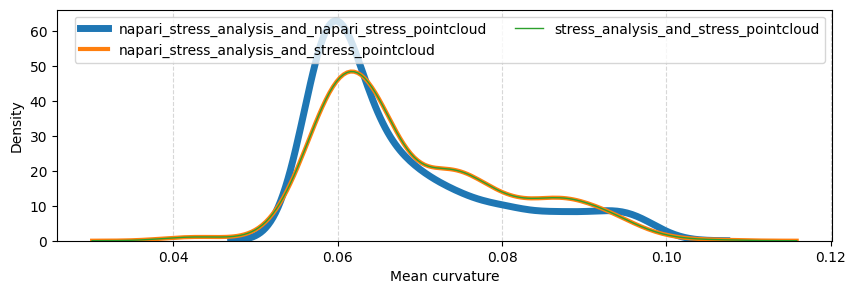
Here, we compare the measured mean curvatures for each of the above-described workflows. We can observe that the mean curvatures for the workflows “napari_stress_analysis_and_stress_pointcloud” and “stress_analysis_and_stress_pointcloud” overlap perfectly. This indicates that any differences between the napari-stress implementation and the legacy version of STRESS are due to the reconstruction of the pointcloud.

mpl.style.use('default')

fig, ax = plt.subplots(figsize=(10,3))
file = 'mean_curvatures.csv'
for idx, directory in enumerate(os.listdir(dataset)):
    if not os.path.isdir(os.path.join(dataset, directory)):
        continue

    mean_curvatures = np.loadtxt(os.path.join(dataset, directory, file))
    sns.kdeplot(data=mean_curvatures, ax=ax, label=directory, linewidth=6-idx*2+1)

ax.set_xlabel('Mean curvature')
ax.grid(which='major', axis='x', linestyle='--', alpha=0.5)

ax.legend(ncols=2)

<matplotlib.legend.Legend at 0x165159b8790>

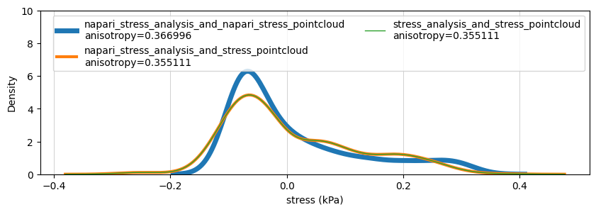
Compare stresses

Here we compare total/cell/tissue stresses for the three workflows:

def calculate_anisotropy(values, alpha=0.05):
    from scipy import stats
    hist_data = np.histogram(values, bins='auto', density=True)
    hist_dist = stats.rv_histogram(hist_data)
    smallest_excluded_value = hist_dist.ppf(alpha)
    largest_excluded_value = hist_dist.ppf(1. - alpha)

    return largest_excluded_value - smallest_excluded_value

fig, ax = plt.subplots(figsize=(10,3))
file = 'total_stress.csv'
idx = 0
for idx, directory in enumerate(os.listdir(dataset)):
    if not os.path.isdir(os.path.join(dataset, directory)):
        continue

    total_stresses = np.loadtxt(os.path.join(dataset, directory, file))
    anisotropy = calculate_anisotropy(total_stresses)
    sns.kdeplot(data=total_stresses, ax=ax, label=directory+'\nanisotropy={:2f}'.format(anisotropy), linewidth=6-idx*2+1)
    ax.set_xlabel('stress (kPa)')
    ax.grid(which='major', axis='x', linestyle='-', linewidth='0.5', color='gray', alpha=0.5)

    ax.legend()
    idx += 1

Ellipsoid

In this section, we repeat the analysis workflow from above for synthetic data of an ellipsoid with major axis lengths of (20, 15, 15).

dataset = os.path.join('.', 'results_ellipsoid')

viewer2 = napari.Viewer()

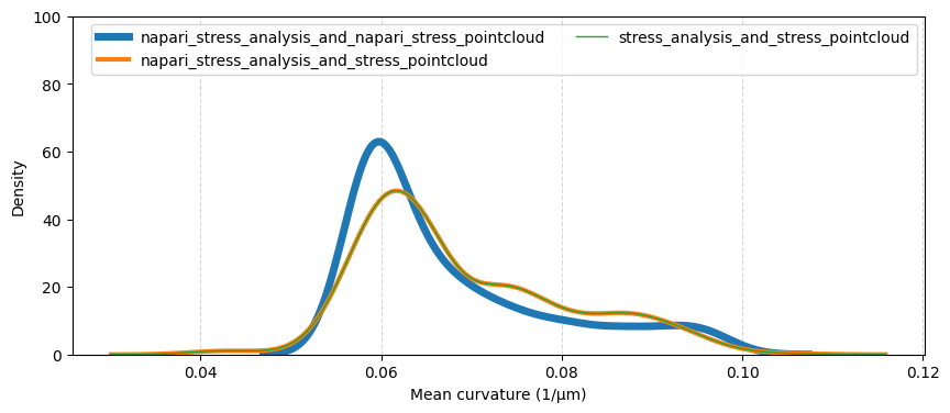
Mean curvatures

We now plot the distribution of mean curvatures on the synthetic ellipsoid for the three experimental workflows described above. It is not clear whether the process of creating the synthetic image data delivers an ellipsoid image with the same major axis lengths which were used to create the initial pointcloud (see this notebook).

Hence, we compare the measured mean curvatures with both the originally used major axis lenghts (20, 15, 15) as well as with the axis lengths of the pointclouds that were recovered with the respective methods:

axis_lengths = (20, 15, 15)
axis_lengths = np.sort(axis_lengths)[::-1]
print('a = {:.2f} px, b = {:.2f} px, c = {:.2f} px'.format(*axis_lengths))

a = 20.00 px, b = 15.00 px, c = 15.00 px

mpl.style.use('default')

fig, ax = plt.subplots(figsize=(10,4))
idx = 0
for idx, directory in enumerate(os.listdir(dataset)):
    if not os.path.exists(os.path.join(dataset, directory, 'mean_curvatures.csv')):
        continue

    mean_curvatures = np.loadtxt(os.path.join(dataset, directory, 'mean_curvatures.csv'))
    sns.kdeplot(data=mean_curvatures, ax=ax, label=directory, linewidth=6-idx*2+1)

ax.set_xlabel('Mean curvature (1/µm)')
ax.grid(which='major', axis='x', linestyle='--', alpha=0.5)
ax.legend(ncols=2)
ax.set_ylim(0, 100)

(0.0, 100.0)

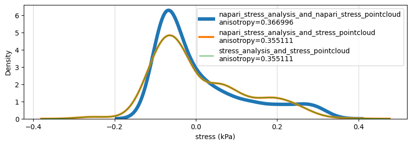
Total stress

We plot the same curve for total stress:

fig, ax = plt.subplots(figsize=(10,3))
file = 'total_stress.csv'
idx = 0
for idx, directory in enumerate(os.listdir(dataset)):
    if not os.path.exists(os.path.join(dataset, directory, file)):
        continue

    total_stresses = np.loadtxt(os.path.join(dataset, directory, file))
    anisotropy = calculate_anisotropy(total_stresses)
    sns.kdeplot(data=total_stresses, ax=ax, label=directory+'\nanisotropy={:2f}'.format(anisotropy), linewidth=6-idx*2+1)
ax.set_xlabel('stress (kPa)')
ax.grid(which='major', axis='x', linestyle='-', linewidth='0.5', color='gray', alpha=0.5)

ax.legend(ncols=2)
ax.set_ylim(0, 10)

(0.0, 10.0)