Analyze everything

This notebook demonstrates how to run a complete STRESS analysis and produce all relevant output graphs. If you want to download this notebook and execute it locally on your machine, download this file as a ipynb Jupyter notebook file and run it in your local python environment using the download button at the top of this page.

import napari_stress
import napari
import numpy as np
from napari_stress import reconstruction, measurements, TimelapseConverter, utils, stress_backend, plotting
import os
import datetime

from skimage import io

import pandas as pd
import seaborn as sns
import matplotlib.pyplot as plt
import matplotlib as mpl

import yaml

viewer = napari.Viewer(ndisplay=3)

reconstruction_parameters = None
measurement_parameters = None

Load the data

Replace the following code with the commented out part (and remove the rest) below to load your own data for analysis:

image = napari_stress.get_droplet_4d()[0][0]
image.shape
filename = None

## Replace this code with a command to import your data. Example:
# filename = 'path/to/data.tif'
# image = io.imread(filename)

Data dimensions

You need to set a few parameters pertaining to your data:

voxel_size_x = 2.078  # microns
voxel_size_y = 2.078  # microns
voxel_size_z = 3.998  # microns
target_voxel_size = 2.078  # microns
time_step = 3  # minutes

viewer.add_image(image, scale=[voxel_size_z, voxel_size_y, voxel_size_x], name='droplet')

<Image layer 'droplet' at 0x19610584bb0>

Analysis parameters

In case you ran the reconstruction previously interactively from the napari viewer (as explained here) and exported the settings, you can import the settings here, too. To do so, simply uncomment the line below (remove the #) and provide the path to the saved settings file:

# reconstruction_parameters = utils.import_settings(file_name='path/of/reconstruction/settings.yaml')
# measurement_parameters = utils.import_settings(file_name='path/of/measurement/settings.yaml')

If you used a parameter file, you can skip the next step. Otherwise, use this cell to provide the necessary parameters for the reconstruction and the measurement. The parameters are explained here:

• Reconstruction

• Measurement

If you used the previous cell to import some parameters, skip the next cell or delete it.

reconstruction_parameters = {
    'voxelsize': np.asarray([voxel_size_z, voxel_size_y, voxel_size_x]),
    'target_voxelsize': target_voxel_size,
    'smoothing_sigma': 1,
    'n_smoothing_iterations': 15,
    'n_points': 256,
    'n_tracing_iterations': 3,
    'resampling_length': 1,
    'fit_type': 'fancy',   # can be 'fancy' or 'quick'
    'edge_type': 'interior',   # can be 'interior' or 'surface'
    'trace_length': 20,
    'sampling_distance': 0.5,
    'interpolation_method':  'cubic',  # can be 'linear' 'cubic' or 'nearest'
    'outlier_tolerance': 1.5,
    'remove_outliers': True,
    'return_intermediate_results': True}

measurement_parameters = {
    'max_degree': 20,  # spherical harmonics degree
    'n_quadrature_points': 590,  # number of quadrature points to measure on (maximum is 5810)
    'gamma': 3.3}  # interfacial tension of droplet
alpha = 0.05  # lower and upper boundary in cumulative distribution function which should be used to calculate the stress anisotropy

Hint: If you are working with timelapse data, it is recommended to use parallel computation to speed up the analysis.

parallelize = True

Analysis

n_frames = image.shape[0]

We run the reconstruction and the stress analysis:

results_reconstruction = reconstruction.reconstruct_droplet(image, **reconstruction_parameters, use_dask=parallelize)

for res in results_reconstruction:
    layer = napari.layers.Layer.create(res[0], res[1], res[2])
    viewer.add_layer(layer)

Dask client up and running <Client: 'tcp://127.0.0.1:50124' processes=4 threads=4, memory=31.96 GiB>  Log: http://127.0.0.1:8787/status

_ = stress_backend.lbdv_info(Max_SPH_Deg=measurement_parameters['max_degree'],
                             Num_Quad_Pts=measurement_parameters['n_quadrature_points'])

input_data = viewer.layers['Droplet pointcloud (smoothed)'].data
results_stress_analysis = measurements.comprehensive_analysis(input_data, **measurement_parameters,
                                                              use_dask=parallelize)

for res in results_stress_analysis:
    layer = napari.layers.Layer.create(res[0], res[1], res[2])
    viewer.add_layer(layer)

Dask client already running <Client: 'tcp://127.0.0.1:50124' processes=4 threads=4, memory=31.96 GiB>  Log: http://127.0.0.1:8787/status

To get an idea about the returned outputs and which is stored in which layer, let’s print them:

for res in results_stress_analysis:
    print('-->', res[1]['name'])
    if 'metadata' in res[1].keys():
        for key in res[1]['metadata'].keys():
            print('\t Metadata: ', key)
    if 'features' in res[1].keys():
        for key in res[1]['features'].keys():
            print('\t Features: ', key)

--> Result of fit spherical harmonics (deg = 20)
	 Metadata:  Elipsoid_deviation_contribution_matrix
	 Metadata:  frame
	 Features:  fit_residue
	 Features:  frame
--> Result of expand points on ellipsoid
	 Features:  fit_residue
	 Features:  frame
--> Result of least squares ellipsoid
--> Result of lebedev quadrature on ellipsoid
	 Metadata:  Tissue_stress_tensor_cartesian
	 Metadata:  Tissue_stress_tensor_elliptical
	 Metadata:  Tissue_stress_tensor_elliptical_e1
	 Metadata:  Tissue_stress_tensor_elliptical_e2
	 Metadata:  Tissue_stress_tensor_elliptical_e3
	 Metadata:  stress_ellipsoid_anisotropy_e12
	 Metadata:  stress_ellipsoid_anisotropy_e23
	 Metadata:  stress_ellipsoid_anisotropy_e13
	 Metadata:  angle_ellipsoid_cartesian_e1_x1
	 Metadata:  angle_ellipsoid_cartesian_e1_x2
	 Metadata:  angle_ellipsoid_cartesian_e1_x3
	 Metadata:  stress_tissue_anisotropy
	 Metadata:  frame
	 Features:  mean_curvature
	 Features:  stress_tissue
	 Features:  frame
--> Result of lebedev quadrature (droplet)
	 Metadata:  Gauss_Bonnet_relative_error
	 Metadata:  Gauss_Bonnet_error
	 Metadata:  Gauss_Bonnet_error_radial
	 Metadata:  Gauss_Bonnet_relative_error_radial
	 Metadata:  H0_volume_integral
	 Metadata:  H0_arithmetic
	 Metadata:  H0_surface_integral
	 Metadata:  S2_volume_integral
	 Metadata:  stress_cell_nearest_pair_anisotropy
	 Metadata:  stress_cell_nearest_pair_distance
	 Metadata:  stress_cell_all_pair_anisotropy
	 Metadata:  stress_cell_all_pair_distance
	 Metadata:  frame
	 Features:  mean_curvature
	 Features:  difference_mean_curvature_cartesian_radial_manifold
	 Features:  stress_cell
	 Features:  stress_total
	 Features:  stress_total_radial
	 Features:  stress_cell_extrema
	 Features:  stress_total_extrema
	 Features:  frame
--> Total stress: Geodesics maxima -> nearest minima
--> Total stress: Geodesics minima -> nearest maxima
--> Cell stress: Geodesics maxima -> nearest minima
--> Cell stress: Geodesics minima -> nearest maxima
--> stress_autocorrelations
	 Metadata:  autocorrelations_spatial_total
	 Metadata:  autocorrelations_spatial_cell
	 Metadata:  autocorrelations_spatial_tissue
	 Metadata:  frame

To make handling further down easier, we store all data and metadata in a few simple dataframes

# Compile data
df_over_time, df_nearest_pairs, df_all_pairs, df_autocorrelations = utils.compile_data_from_layers(
    results_stress_analysis, n_frames=n_frames, time_step=time_step)

Visualization

In this section, we will plot some interesting results and save the data to disk. The file location will be at the

%%capture
figures_dict = plotting.create_all_stress_plots(
    results_stress_analysis,
    time_step=time_step,
    n_frames=n_frames
)

mpl.style.use('default')
colormap_time = 'flare'
if filename is not None:
    filename_without_ending = os.path.basename(filename).split('.')[0]
    save_directory = os.path.join(os.path.dirname(filename), filename_without_ending + '_' + datetime.datetime.now().strftime('%Y-%m-%d_%H-%M-%S'))
else: 
    save_directory = os.path.join(os.getcwd(), 'results_' + datetime.datetime.now().strftime('%Y-%m-%d_%H-%M-%S'))

if not os.path.exists(save_directory):
    os.makedirs(save_directory)

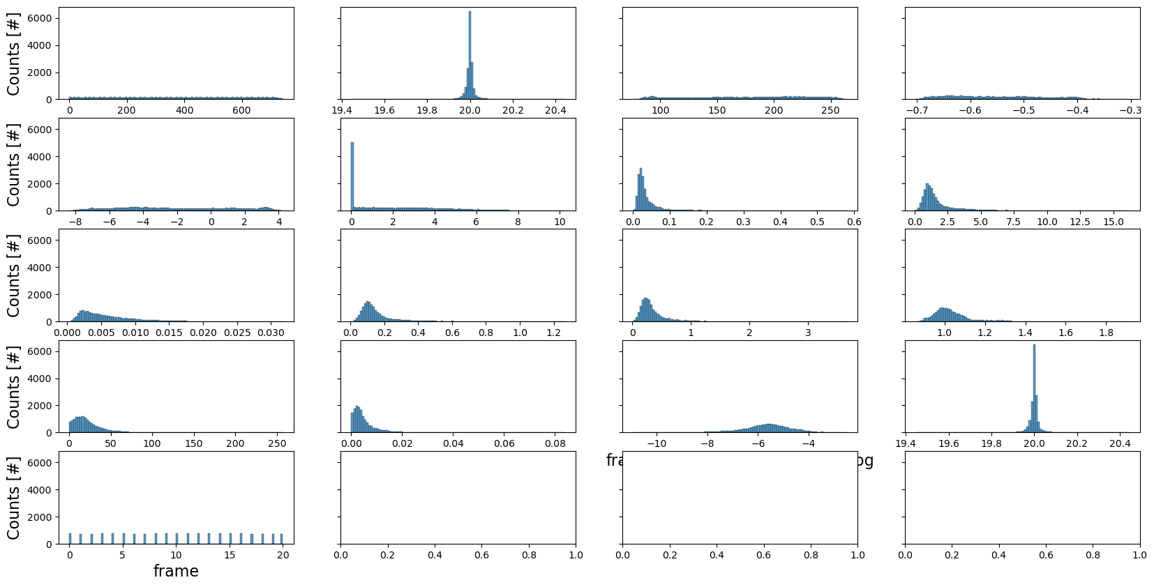
Fit errors

We first show all the errors that were calculated during the pointcloud refinement:

fit_error_df = pd.DataFrame(results_reconstruction[3][1]['features'].reset_index())
fit_error_df

	index	center	amplitude	slope	background_slope	offset	center_err	amplitude_err	slope_err	background_slope_err	offset_err	distance_to_nearest_neighbor	mean_squared_error	fraction_variance_unexplained	fraction_variance_unexplained_log	idx_of_border	frame
0	0	20.038063	176.410822	-0.673940	-1.168413	4.609321e-21	0.046695	2.582717	0.012938	0.307859	0.566758	1.099930	20.261058	0.004435	-5.418143	20.038063	0
1	1	20.022966	163.568899	-0.638404	0.379437	5.848198e-20	0.047042	2.414873	0.011207	0.275440	0.485870	1.096523	6.302603	0.001248	-6.686067	20.022966	0
2	2	20.025295	193.242245	-0.673258	-2.377362	1.104042e-18	0.044560	2.653223	0.012399	0.321607	0.599573	1.118846	33.819470	0.007118	-4.945105	20.025295	0
3	3	20.025143	163.229563	-0.641114	0.257542	1.242458e-21	0.047908	2.453894	0.011555	0.280890	0.497471	1.031137	10.036452	0.002015	-6.207211	20.025143	0
4	4	20.003009	176.166124	-0.670780	-0.900823	3.622026e-20	0.048619	2.688943	0.013216	0.320005	0.577818	1.076207	10.774460	0.002298	-6.075505	20.003009	0
...	...	...	...	...	...	...	...	...	...	...	...	...	...	...	...	...	...
15364	725	19.998927	197.392632	-0.627527	-3.770612	3.676951e-01	0.018876	0.962403	0.004785	0.103900	0.237937	1.031561	17.373360	0.003571	-5.634947	19.998927	20
15365	726	20.040552	171.129640	-0.677093	-1.781867	3.194370e-14	0.029979	1.459065	0.009372	0.152425	0.390491	1.131636	18.176025	0.003844	-5.561195	20.040552	20
15366	727	19.995654	179.672688	-0.667468	-2.447113	6.488004e-22	0.025294	1.271959	0.007641	0.134078	0.340907	1.085043	15.459548	0.003339	-5.702091	19.995654	20
15367	728	19.992411	192.269531	-0.652320	-3.107330	1.823652e-16	0.023571	1.247022	0.006770	0.131471	0.335464	1.074869	19.429097	0.003838	-5.562913	19.992411	20
15368	729	20.031783	169.546593	-0.675959	-1.751943	1.263994e-20	0.030450	1.467567	0.009474	0.153350	0.391583	NaN	19.560836	0.004306	-5.447669	20.031783	20

15369 rows × 17 columns

fig, axes = plt.subplots(ncols=4, nrows=len(fit_error_df.columns)//4+1, figsize=(20, 10), sharey=True)
axes = axes.flatten()
for idx, column in enumerate(fit_error_df.columns):
    ax = axes[idx]

    sns.histplot(data=fit_error_df, x=column, ax=ax, bins=100)
    ax.set_xlabel(column, fontsize=16)
    ax.set_ylabel('Counts [#]', fontsize=16)

if save_directory is not None:
    fig.savefig(os.path.join(save_directory, 'fit_error_reconstruction.png'), dpi=300)

Spherical harmonics

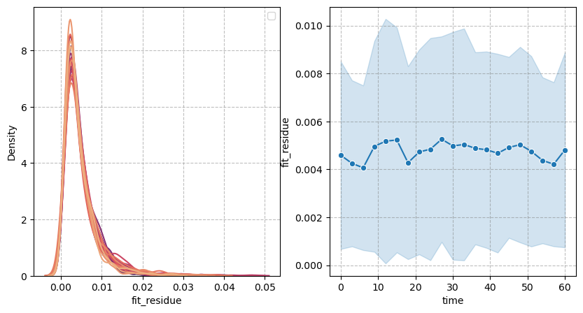
Fit residue

We now show the errors made when approximating the reconstructed pointcloud with the spherical harmonics:

figure = figures_dict['Figure_reside']
if save_directory is not None:
    figure['figure'].savefig(os.path.join(save_directory, figure['path']), dpi=300)

figure['figure']

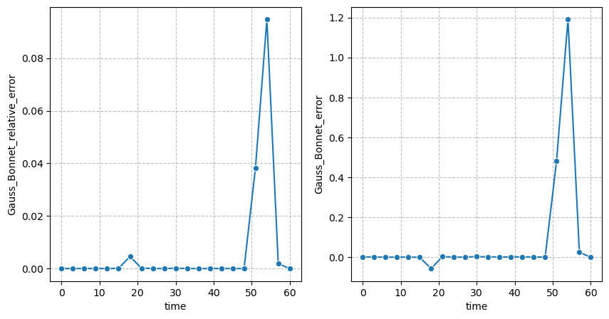
Fit quality

We can quantify the quality of the extracted pointcloud by using the absolute and relative Gauss-Bonnet errors:

figure = figures_dict['fig_GaussBonnet_error']
if save_directory is not None:
    figure['figure'].savefig(os.path.join(save_directory, figure['path']), dpi=300)

figure['figure']

Curvature

We next show mean curvature histograms and averages over time:

figure = figures_dict['fig_mean_curvature']
if save_directory is not None:
    figure['figure'].savefig(os.path.join(save_directory, figure['path']), dpi=300)

figure['figure'].axes[0].set_xlabel("Mean curvature [$mm^{-1}$]", fontsize=16)

figure['figure'].axes[1].set_ylabel("Mean curvature [$mm^{-1}$]", fontsize=16)
figure['figure'].axes[1].set_xlabel("Time [min]", fontsize=16)

figure['figure']

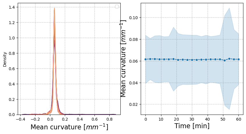
figure = figures_dict['fig_total_stress']
if save_directory is not None:
    figure['figure'].savefig(os.path.join(save_directory, figure['path']), dpi=300)

figure['figure']

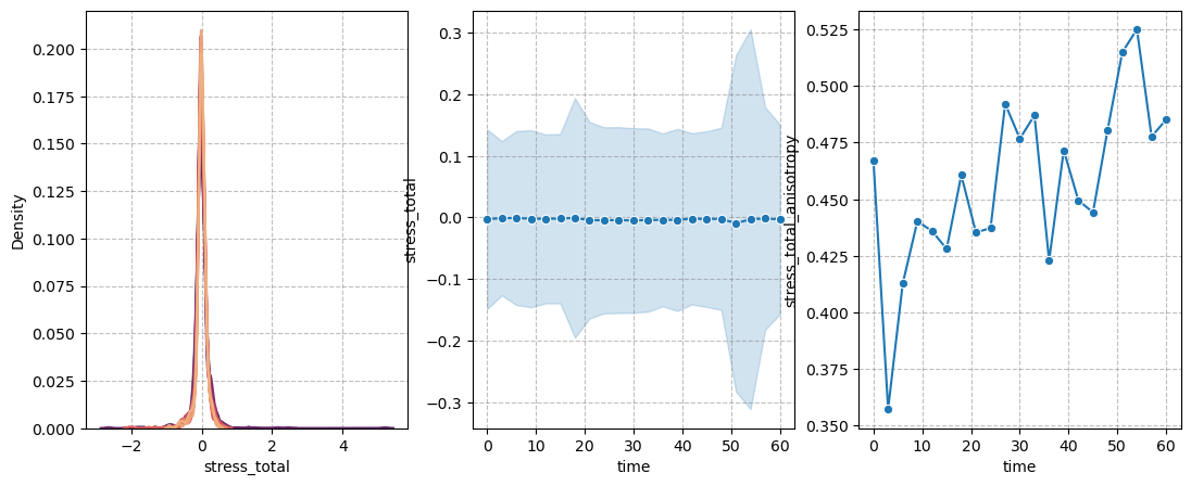
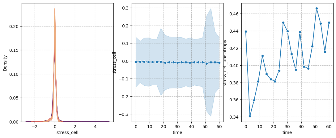
figure = figures_dict['fig_cell_stress']
if save_directory is not None:
    figure['figure'].savefig(os.path.join(save_directory, figure['path']), dpi=300)

figure['figure']

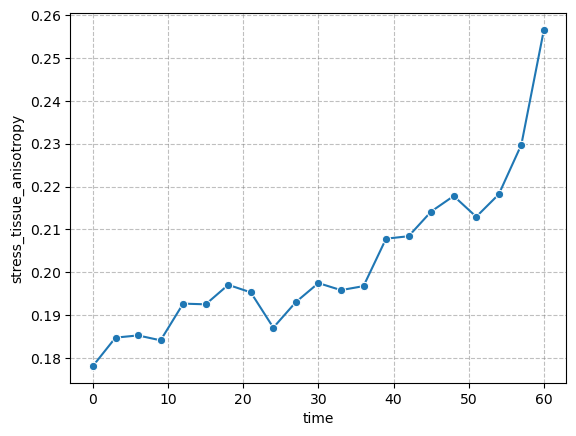
Tissue-scale stresses

figure = figures_dict['fig_tissue_stress']
if save_directory is not None:
    figure['figure'].savefig(os.path.join(save_directory, figure['path']), dpi=300)

figure['figure']

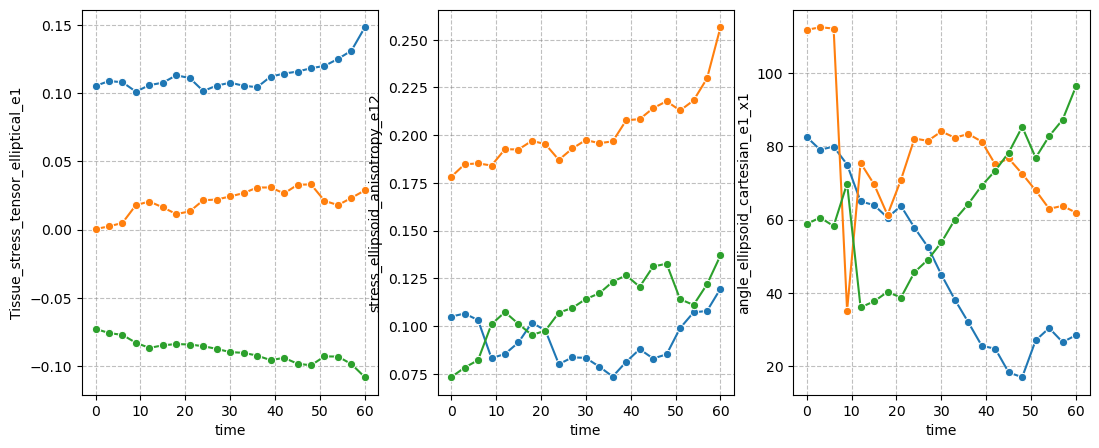
Stress along axes

figure = figures_dict['fig_stress_tensor']
if save_directory is not None:
    figure['figure'].savefig(os.path.join(save_directory, figure['path']), dpi=300)

figure['figure']

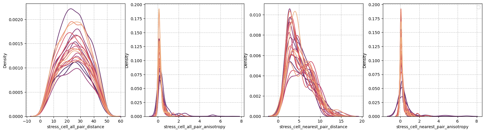
Extrema analysis

figure = figures_dict['fig_all_pairs']
if save_directory is not None:
    figure['figure'].savefig(os.path.join(save_directory, figure['path']), dpi=300)

figure['figure']

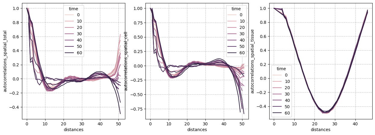
Autocorrelations: Spatial

figure = figures_dict['fig_spatial_autocorrelation']
if save_directory is not None:
    figure['figure'].savefig(os.path.join(save_directory, figure['path']), dpi=300)

figure['figure']

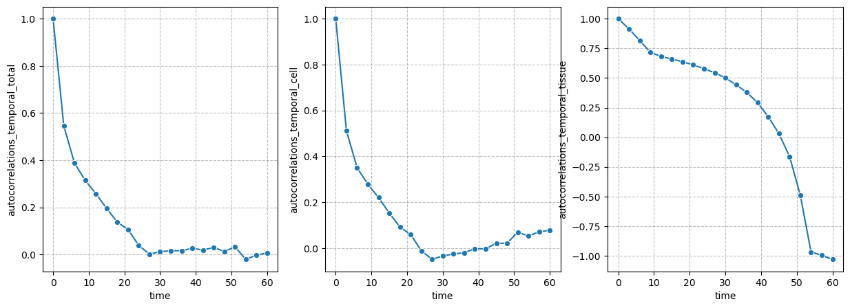
Autocorrelations: Temporal

figure = figures_dict['fig_temporal_autocorrelation']
if save_directory is not None:
    figure['figure'].savefig(os.path.join(save_directory, figure['path']), dpi=300)

figure['figure']

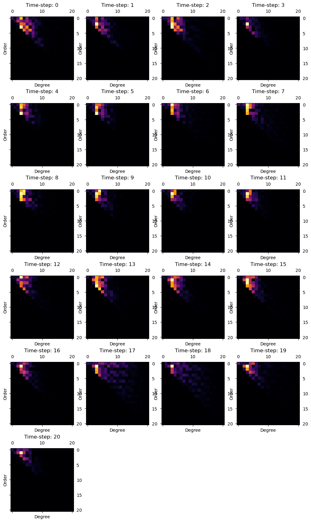
Ellipsoid deviation

figure = figures_dict['fig_ellipsoid_contribution']
if save_directory is not None:
    figure['figure'].savefig(os.path.join(save_directory, figure['path']), dpi=300)

figure['figure']

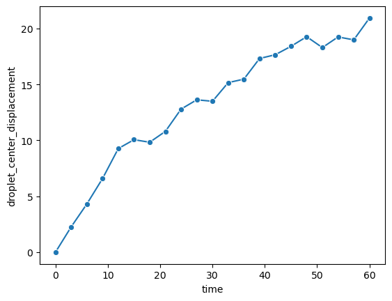
Droplet movement

This analyzes how much the center of the droplet moves over time.

Converter = TimelapseConverter()
list_of_points = Converter.data_to_list_of_data(results_reconstruction[3][0], layertype=napari.types.PointsData)
center = [np.mean(points, axis=0) for points in list_of_points]
center_displacement = np.asarray([np.linalg.norm(center[t] - center[0]) for t in range(n_frames)])
df_over_time['droplet_center_displacement'] =  center_displacement * target_voxel_size

sns.lineplot(data=df_over_time, x='time', y='droplet_center_displacement', marker='o')

<Axes: xlabel='time', ylabel='droplet_center_displacement'>

Export data

We first agregate the data from the spatial autocorrelations in a separate dataframe. This dataframe has a column for autocorrelations of total, cell and tissue-scale stresses.

df_to_export = pd.DataFrame()
for col in df_over_time.columns:
    if isinstance(df_over_time[col].iloc[0], np.ndarray):
        continue
    if np.stack(df_over_time[col].to_numpy()).shape == (n_frames,):
        df_to_export[col] = df_over_time[col].to_numpy()

df_to_export.to_csv(os.path.join(save_directory, 'results_over_time.csv'), index=False)

We also export the used settings for the analysis into a .yml file:

utils.export_settings(reconstruction_parameters, file_name=os.path.join(save_directory, 'reconstruction_settings.yaml'))
utils.export_settings(measurement_parameters, file_name=os.path.join(save_directory, 'measurement_settings.yaml'))