Spherical harmonics

This notebook demonstrates how to use a set of spherical harmonics functions to approximate pointclouds in 3D.

from napari_stress import approximation
import vedo
import napari
import matplotlib.pyplot as plt

Let’s create some sample surface data which we would like to approximate with a spherical harmonics expansion (SHE), for instance an ellipsoid:

data = vedo.Ellipsoid(axis1=[10, 0, 0], axis2=[0, 20, 0], axis3=[0, 0, 30], pos=[0,0,0])
viewer = napari.Viewer(ndisplay=3)
viewer.add_points(data.vertices, size=0.5, face_color='orange', name='Raw')
napari.utils.nbscreenshot(viewer, canvas_only=True)

Expansion

Now we use the SphericalHarmonicsExpander class to approximate this pointcloud. The important parameter is the max_degree parameter. Higher values for this parameter will tell the function to include spherical harmonic functions of higher orders to approximate the pointcloud and arrive at a better estimation. You’ll see that the approximation of the ellipsoid becomes better with higher order. We start with a low order to demonstrate the effect:

Expander = approximation.SphericalHarmonicsExpander(max_degree=1)
fitted_points = Expander.fit_expand(data.vertices)
print('Mean distance between input points and fitted points: ', Expander.properties['residuals'].mean())

Mean distance between input points and fitted points:  4.417060747478731e-06

viewer.add_points(fitted_points, size=0.5, features={'residuals': Expander.properties['residuals']},
                  face_color='residuals', name=f'Fitted_order={1}', face_colormap='inferno')

viewer.camera.angles = (0, 45, 45)
napari.utils.nbscreenshot(viewer, canvas_only=True)

Now we use a higher order to approximate the ellipsoid. We can see that the remaining approximation error is less localized and more evenly distributed over the surface of the ellipsoid, which indicates a better overall approximation.

Expander = approximation.SphericalHarmonicsExpander(max_degree=15)
fitted_points = Expander.fit_expand(data.vertices)
print('Mean distance between input points and fitted points: ', Expander.properties['residuals'].mean())

Mean distance between input points and fitted points:  2.2754520120179687e-07

viewer.layers['Fitted_order=1'].visible = False
viewer.add_points(fitted_points, size=0.5, features={'residuals': Expander.properties['residuals']},
                  face_color='residuals', name=f'Fitted_order={15}', face_colormap='inferno')

viewer.camera.angles = (0, 45, 45)
napari.utils.nbscreenshot(viewer, canvas_only=True)

Quantification

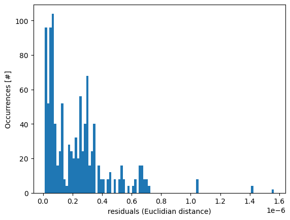
The SphericalHarmonicsExpander allows you to extract a few interesting properties. For instance, it can tell you how well the expansion approximates your input:

fig, ax = plt.subplots()
ax.hist(Expander.properties['residuals'], bins=100)
ax.set_xlabel('residuals (Euclidian distance)')
ax.set_ylabel('Occurrences [#]')

Text(0, 0.5, 'Occurrences [#]')

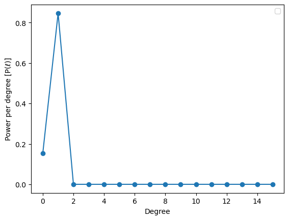
You can also examine the powerspectrum of the expansion. In essence, it tells you, how much quality each degree \(l\) of the expansion adds to the approximation. In the standard case in this implementation, the coordinates \(x\), \(y\) and \(z\) are expanded separately, so a separate powerspectrum is calculated for each of them.

powerspectrum = Expander.properties['power_spectrum']

fig, ax = plt.subplots()
ax.plot(powerspectrum, 'o-')
ax.set_xlabel('Degree')
ax.set_ylabel('Power per degree [P(ℓ)]')
ax.legend()

No artists with labels found to put in legend.  Note that artists whose label start with an underscore are ignored when legend() is called with no argument.

<matplotlib.legend.Legend at 0x1ccb5c42820>

If you want to evaluate all coefficients, this is a bit more complicated.

Mathematical background: A spherical harmonics approximation (a.k.a. expansion) \(f(\theta,\phi)\) can be written as a superposition of multiple single spherical harmonics functions \(Y_l^m(\theta\phi)\) of different degree and order:

\(f(\theta,\phi) = \sum_{l=0}^{\infty} \sum_{m=-l}^{l} f_l^m Y_l^m(\theta\phi)\)

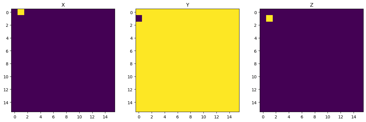
whereas the coefficients \(f_l^m\) determine how much contribution of which degree \(l\) and order \(m\) is needed to achieve the best approximation of the input pointcloud. Currently, napari-stress performs the sperhical harmonics expansion separately for the \(x\), \(y\) and \(z\) direction, hence you’ll receive three distinct shape spectra:

fig, axes = plt.subplots(ncols=3, figsize=(15,5))
axes[0].imshow(Expander.coefficients_[0])
axes[1].imshow(Expander.coefficients_[1])
axes[2].imshow(Expander.coefficients_[2])

axes[0].set_title('X')
axes[1].set_title('Y')
axes[2].set_title('Z')

Text(0.5, 1.0, 'Z')